处理多波段栅格(Sentinel-使用 hndex 并创建索引
来源:dev.to
时间:2024-08-26 11:01:20 137浏览 收藏
本篇文章给大家分享《处理多波段栅格(Sentinel-使用 hndex 并创建索引》,覆盖了文章的常见基础知识,其实一个语言的全部知识点一篇文章是不可能说完的,但希望通过这些问题,让读者对自己的掌握程度有一定的认识(B 数),从而弥补自己的不足,更好的掌握它。
嗨,在之前的博客中,我们讨论了如何使用 h3 索引和 postgresql 对单波段栅格进行栅格分析。在本博客中,我们将讨论如何处理多波段栅格并轻松创建索引。我们将使用 sentinel-2 图像并从处理后的 h3 细胞创建 ndvi 并可视化结果
下载哨兵2数据
我们正在从尼泊尔博卡拉地区的https://apps.sentinel-hub.com/eo-browser/下载sentinel 2数据,只是为了确保湖泊在图像网格中,以便我们可以轻松地验证 ndvi 结果

要下载所有乐队的哨兵图像:
- 您需要创建一个帐户
- 找到您所在区域的图像,选择覆盖您感兴趣区域的网格
- 放大到网格,然后点击右侧竖条上的
 图标
图标 - 之后进入分析选项卡并选择图像格式为 tiff 32 位、高分辨率、wgs1984 格式的所有波段并检查所有波段
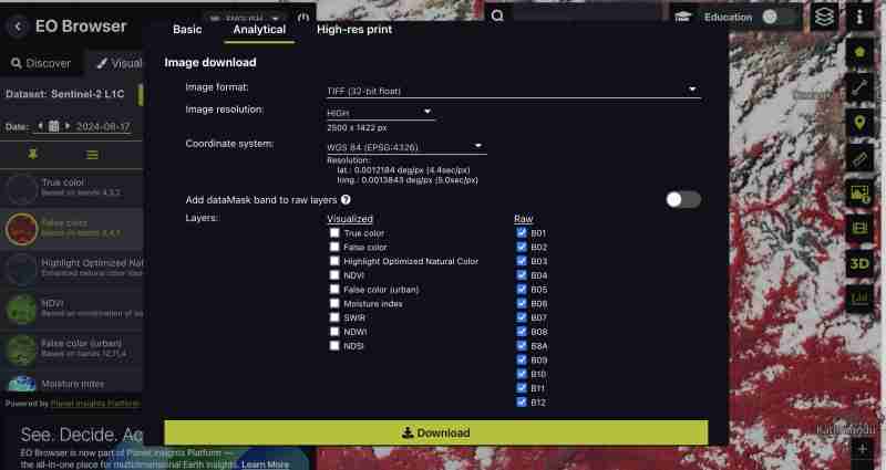
您还可以下载预生成的指数,例如 ndvi、仅假色 tiff 或最适合您需要的特定波段。我们正在下载所有乐队,因为我们想自己进行处理
- 点击下载
预处理
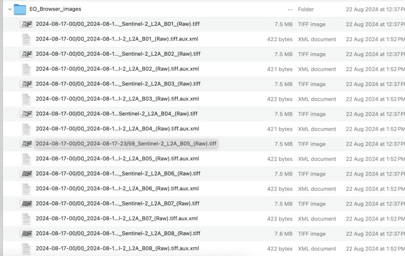
当我们下载原始格式时,我们将所有乐队作为与哨兵分开的 tiff
- 让我们创建一个合成图像:
这可以通过gis工具或gdal来完成
- 使用 gdal_merge:
我们需要将下载的文件重命名为 band1,band2 以避免文件名中出现斜杠
本次练习最多处理频段 9,您可以根据需要选择频段
gdal_merge.py -separate -o sentinel2_composite.tif band1.tif band2.tif band3.tif band4.tif band5.tif band6.tif band7.tif band8.tif band9.tif
- 使用 qgis :
- 将所有单独的波段加载到 qgis
- 转到光栅 > 杂项 > 合并
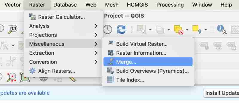
- 合并时,您需要确保选中“将每个输入文件放入 sep band”
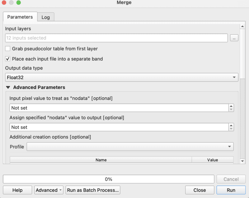
- 现在将合并的 tiff 作为复合材料导出到原始 geotiff
家政
- 确保您的图像采用 wgs1984 在我们的例子中,图像已经是 ws1984,所以不需要转换
- 确保您没有任何 nodata 如果有则用 0 填充
gdalwarp -overwrite -dstnodata 0 "$input_file" "${output_file}_nodata.tif"
- 最后确保你的输出图像是cog
gdal_translate -of cog "$input_file" "$output_file"
我正在使用 cog2h3 repo 中提供的 bash 脚本来自动化这些
sudo bash pre.sh sentinel2_composite.tif
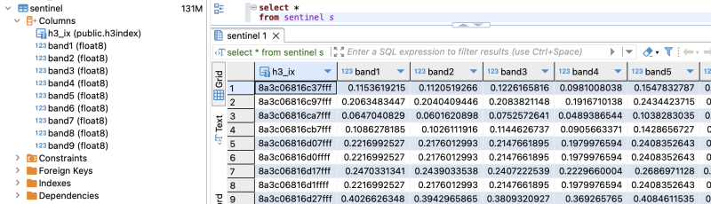
h3细胞的处理和创建
现在,我们终于完成了预处理脚本,让我们继续计算复合齿轮图像中每个波段的 h3 单元格
- 安装cog2h3
pip install cog2h3
- 导出您的数据库凭据
export database_url="postgresql://user:password@host:port/database"
- 奔跑
我们对此哨兵图像使用分辨率 10,但是您还会在脚本本身中看到,它将打印栅格的最佳分辨率,使 h3 单元小于栅格中的最小像素。
cog2h3 --cog sentinel2_composite_preprocessed.tif --table sentinel --multiband --res 10
我们花了一分钟的时间来计算结果并将结果存储在 postgresql 中
日志:
2024-08-24 08:39:43,233 - info - starting processing
2024-08-24 08:39:43,234 - info - cog file already exists at sentinel2_composite_preprocessed.tif
2024-08-24 08:39:43,234 - info - processing raster file: sentinel2_composite_preprocessed.tif
2024-08-24 08:39:43,864 - info - determined min fitting h3 resolution for band 1: 11
2024-08-24 08:39:43,865 - info - resampling original raster to: 200.786148m
2024-08-24 08:39:44,037 - info - resampling done for band 1
2024-08-24 08:39:44,037 - info - new native h3 resolution for band 1: 10
2024-08-24 08:39:44,738 - info - calculation done for res:10 band:1
2024-08-24 08:39:44,749 - info - determined min fitting h3 resolution for band 2: 11
2024-08-24 08:39:44,749 - info - resampling original raster to: 200.786148m
2024-08-24 08:39:44,757 - info - resampling done for band 2
2024-08-24 08:39:44,757 - info - new native h3 resolution for band 2: 10
2024-08-24 08:39:45,359 - info - calculation done for res:10 band:2
2024-08-24 08:39:45,366 - info - determined min fitting h3 resolution for band 3: 11
2024-08-24 08:39:45,366 - info - resampling original raster to: 200.786148m
2024-08-24 08:39:45,374 - info - resampling done for band 3
2024-08-24 08:39:45,374 - info - new native h3 resolution for band 3: 10
2024-08-24 08:39:45,986 - info - calculation done for res:10 band:3
2024-08-24 08:39:45,994 - info - determined min fitting h3 resolution for band 4: 11
2024-08-24 08:39:45,994 - info - resampling original raster to: 200.786148m
2024-08-24 08:39:46,003 - info - resampling done for band 4
2024-08-24 08:39:46,003 - info - new native h3 resolution for band 4: 10
2024-08-24 08:39:46,605 - info - calculation done for res:10 band:4
2024-08-24 08:39:46,612 - info - determined min fitting h3 resolution for band 5: 11
2024-08-24 08:39:46,612 - info - resampling original raster to: 200.786148m
2024-08-24 08:39:46,619 - info - resampling done for band 5
2024-08-24 08:39:46,619 - info - new native h3 resolution for band 5: 10
2024-08-24 08:39:47,223 - info - calculation done for res:10 band:5
2024-08-24 08:39:47,230 - info - determined min fitting h3 resolution for band 6: 11
2024-08-24 08:39:47,230 - info - resampling original raster to: 200.786148m
2024-08-24 08:39:47,239 - info - resampling done for band 6
2024-08-24 08:39:47,239 - info - new native h3 resolution for band 6: 10
2024-08-24 08:39:47,829 - info - calculation done for res:10 band:6
2024-08-24 08:39:47,837 - info - determined min fitting h3 resolution for band 7: 11
2024-08-24 08:39:47,837 - info - resampling original raster to: 200.786148m
2024-08-24 08:39:47,845 - info - resampling done for band 7
2024-08-24 08:39:47,845 - info - new native h3 resolution for band 7: 10
2024-08-24 08:39:48,445 - info - calculation done for res:10 band:7
2024-08-24 08:39:48,453 - info - determined min fitting h3 resolution for band 8: 11
2024-08-24 08:39:48,453 - info - resampling original raster to: 200.786148m
2024-08-24 08:39:48,461 - info - resampling done for band 8
2024-08-24 08:39:48,461 - info - new native h3 resolution for band 8: 10
2024-08-24 08:39:49,046 - info - calculation done for res:10 band:8
2024-08-24 08:39:49,054 - info - determined min fitting h3 resolution for band 9: 11
2024-08-24 08:39:49,054 - info - resampling original raster to: 200.786148m
2024-08-24 08:39:49,062 - info - resampling done for band 9
2024-08-24 08:39:49,063 - info - new native h3 resolution for band 9: 10
2024-08-24 08:39:49,647 - info - calculation done for res:10 band:9
2024-08-24 08:39:51,435 - info - converting h3 indices to hex strings
2024-08-24 08:39:51,906 - info - overall raster calculation done in 8 seconds
2024-08-24 08:39:51,906 - info - creating or replacing table sentinel in database
2024-08-24 08:40:03,153 - info - table sentinel created or updated successfully in 11.25 seconds.
2024-08-24 08:40:03,360 - info - processing completed
分析
现在我们的数据已经在 postgresql 中了,让我们做一些分析吧
- 验证我们是否拥有处理过的所有频段(记住我们处理的是频段 1 到 9)
select *
from sentinel
- 计算每个细胞的 ndvi
explain analyze
select h3_ix , (band8-band4)/(band8+band4) as ndvi
from public.sentinel
查询计划:
query plan                                                                                                       |
-----------------------------------------------------------------------------------------------------------------+
seq scan on sentinel  (cost=0.00..28475.41 rows=923509 width=16) (actual time=0.014..155.049 rows=923509 loops=1)|
planning time: 0.080 ms                                                                                          |
execution time: 183.764 ms                                                                                       |
正如您在此处看到的那样,该区域中的所有行的计算都是即时的。对于所有其他索引都是如此,您可以使用 h3_ix 主键计算与其他表的复杂索引连接,并从中导出有意义的结果,而不必担心,因为 postgresql 能够处理复杂的查询和表连接。
可视化和验证
让我们可视化并验证计算的索引是否正确
- 创建表格(用于在 qgis 中可视化)
create table ndvi_sentinel
as(
select h3_ix , (band8-band4)/(band8+band4) as ndvi
from public.sentinel )
- 让我们添加几何图形来可视化 h3 细胞 这仅是在 qgis 中可视化所必需的,如果您自己构建一个最小的 api,则不需要它,因为您可以直接从查询构造几何图形
alter table ndvi_sentinel
add column geometry geometry(polygon, 4326)
generated always as (h3_cell_to_boundary_geometry(h3_ix)) stored;
- 在几何体上创建索引
create index on ndvi_sentinel(geometry);
- 在qgis中连接数据库并根据ndvi值可视化表格 让我们获取费瓦湖或云附近的区域
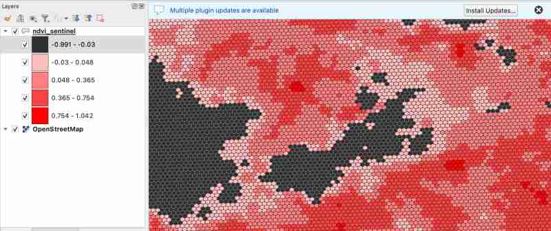
据我们所知,-1.0 到 0.1 之间的值应该代表深水或浓密的云层
让我们看看这是否属实(使第一个类别透明以查看底层图像)
- 检查云:
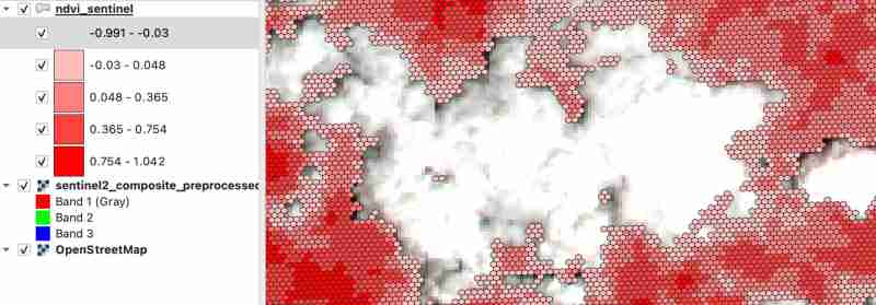
- 检查湖
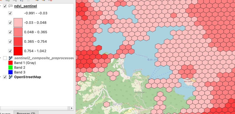
由于湖周围有云,因此附近的田野被云覆盖,这是有道理的

感谢您的阅读!下一篇博客见
今天关于《处理多波段栅格(Sentinel-使用 hndex 并创建索引》的内容介绍就到此结束,如果有什么疑问或者建议,可以在golang学习网公众号下多多回复交流;文中若有不正之处,也希望回复留言以告知!
-
501 收藏
-
501 收藏
-
501 收藏
-
501 收藏
-
501 收藏
-
文章 · python教程 | 2天前 | 日志 · 工程化 · 异步编程 · 故障排查 · 可观测性 · Python教程 · Python 异步任务 可观测性 logging contextvars 生产实践 QueueHandler QueueListener request_id JSON日志189 收藏
-
文章 · python教程 | 3天前 | 依赖管理 · 工程化 · CI · 生产实践 · Python教程 · 打包发布 · Python build 依赖管理 twine wheel 打包发布 pyproject.toml dependency-groups pylock.toml sdist479 收藏
-
文章 · python教程 | 3天前 | WEB开发 · 工程化 · 配置管理 · flask · 生产实践 · Python教程 · Python Flask G 配置管理 请求上下文 应用上下文 生产实践 current_app teardown app factory257 收藏
-
文章 · python教程 | 3天前 | ORM · Django · 异步编程 · 生产实践 · Python教程 · 后端开发 · Python Django 性能优化 orm 事务 ASGI 生产实践 async view sync_to_async310 收藏
-
文章 · python教程 | 3天前 | 性能优化 · 异步编程 · fastapi · 生产实践 · Python教程 · API服务 · Python API服务 FastAPI asyncio httpx 生产实践 lifespan BackgroundTasks run_in_threadpool411 收藏
-
文章 · python教程 | 4天前 | 工程化 · 自动化测试 · pytest · CI · 生产实践 · Python教程 · Python CI pytest fixture tmp_path monkeypatch pytest-xdist 测试稳定性303 收藏
-
文章 · python教程 | 4天前 | sqlalchemy · 异步编程 · fastapi · 生产实践 · Python教程 · Python 连接池 FastAPI sqlalchemy asyncio AsyncSession340 收藏
-
文章 · python教程 | 4天前 | 性能优化 · fastapi · 生产实践 · Python教程 · Pydantic · Python 性能优化 FastAPI Pydantic v2 TypeAdapter validate_json342 收藏
-
文章 · python教程 | 4天前 | 性能优化 · gil · 生产实践 · Python教程 · CPython · Python 性能优化 线程安全 gil CPython free-threaded381 收藏
-
文章 · python教程 | 5天前 | 异步编程 · fastapi · 后端架构 · Python教程 · asyncio · Python 异步编程 FastAPI asyncio TaskGroup 生产实践496 收藏
-
447 收藏
-
189 收藏
-

- 前端进阶之JavaScript设计模式
- 设计模式是开发人员在软件开发过程中面临一般问题时的解决方案,代表了最佳的实践。本课程的主打内容包括JS常见设计模式以及具体应用场景,打造一站式知识长龙服务,适合有JS基础的同学学习。
- 立即学习 543次学习
-

- GO语言核心编程课程
- 本课程采用真实案例,全面具体可落地,从理论到实践,一步一步将GO核心编程技术、编程思想、底层实现融会贯通,使学习者贴近时代脉搏,做IT互联网时代的弄潮儿。
- 立即学习 516次学习
-

- 简单聊聊mysql8与网络通信
- 如有问题加微信:Le-studyg;在课程中,我们将首先介绍MySQL8的新特性,包括性能优化、安全增强、新数据类型等,帮助学生快速熟悉MySQL8的最新功能。接着,我们将深入解析MySQL的网络通信机制,包括协议、连接管理、数据传输等,让
- 立即学习 500次学习
-

- JavaScript正则表达式基础与实战
- 在任何一门编程语言中,正则表达式,都是一项重要的知识,它提供了高效的字符串匹配与捕获机制,可以极大的简化程序设计。
- 立即学习 487次学习
-

- 从零制作响应式网站—Grid布局
- 本系列教程将展示从零制作一个假想的网络科技公司官网,分为导航,轮播,关于我们,成功案例,服务流程,团队介绍,数据部分,公司动态,底部信息等内容区块。网站整体采用CSSGrid布局,支持响应式,有流畅过渡和展现动画。
- 立即学习 485次学习